Paper reading: "Estimating individual treatment effect: generalization bounds and algorithms"
Uri Shalit, Fredrik D. Johansson, David Sontag
Causal inference tasks are often focused on estimating the average effect of a treatment across a population—the ATE (average treatment effect) and the ATT (average treatment effect on the treated). In this paper, the researchers instead focus on Individual Treatment Effect (ITE). In reality many decisions are in fact made on an individual level—e.g., how should a doctor treat an individual patient with symptoms far from the average case?—making the goal of bounding ITE error a highly-desirable one.
The bounds in this paper are proven in the context of an assumption known as strong ignorability, which means (1.) we're assuming there are no hidden confounders—every feature that has a causal impact on the outcome $Y$ is observed in either the treatment $t$ or the covariates $x$—and (2.) $0 < p(t = 1) < 1$ over the entire distribution, meaning we don't have to worry about problems of overlap between treatment and control.
Intuition
How should we think about the task of bounding ITE error? Here is one way: we can fit one model to our data that estimates the outcome of the treated group ($t = 1$) and another that estimates the outcome of the control group ($t = 0$). Call these two functions $m_1(x) = \mathbb{E}[Y_1 \mid x]$ and $m_0(x) = \mathbb{E}[Y_0 \mid x]$, respectively. Then the ITE function—the effect of the treatment on an individual with covariates $x$—is given by $m_1(x) - m_0(x)$. $m_0$ and $m_1$ are just ordinary estimators, so we can talk about their generalization errors using existing statistical theory.
But there is an additional source of error we haven't yet accounted for: the samples that $m_1$ and $m_0$ fit are drawn from different distributions $p(Y_1, x \mid t=1)$ and $p(Y_0, x \mid t=0)$. This is what makes causal inference hard: the treated and untreated groups are fundamentally different, so a model that can predict the outcome of an untreated patient with high accuracy might still perform poorly when it comes to predicting the counterfactual outcome that would have occurred in a treated patient if they had not been treated. Somehow, we must also account for this error.
Results
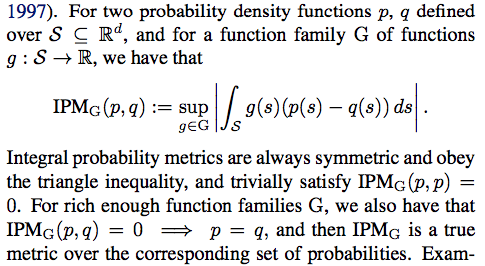
The researchers show that this additional error is bounded by a distance metric between probability distributions called the Integral Probability Metric:
(Recall, or look up on Wikipedia like me, that a metric is just a function that defines a non-negative distance between every two elements of a set, and satisfies a few other conditions like the triangle inequality.)
The bound—expressed as expected Precision in Estimation of Heterogeneous Effect (PEHE), the expected square error of the ITE estimator—is based on a representation function $\Phi$ that maps our data $x$ to some representation space. (This can be thought of as learning some vector embeddings for our data $x$). In the below formulation, $\epsilon_F$ is the factual error—the generalization error of our estimators $m_t$ based on the data we observed. $\epsilon_{CF}$ is the counterfactual error, which we can't actually estimate, since by definition we don't observe counterfactuals. Instead, we bound the counterfactual error with (a constant factor $B_\Phi$ multiplied by) the Integral Probability Metric distance between $p_{\Phi}^{t=1}$ and $p_{\Phi}^{t=0}$, the distributions of the treated and untreated data in representation space.
We can even incorporate the IPM term into our loss function to encourage the neural network to find representations that minimize the distribution distance!
Shalit et. al. call their algorithm Counterfactual Regression, and the version without the IPM regularization "Treatment-Agnostic Representation Network (TARNet)".
Experiments
As usual, evaluating causal inference algorithms is hard because real-world datasets have no ground truth! In this case the researchers evaluate their new algorithm on a "semi-synthetic" Infant Health and Development Program (IDHP) dataset and the ubiquitous LaLonde Jobs dataset. The Jobs dataset consists of both a randomized and non-randomized component, making it a popular choice for causal inference model evaluation.
Models are evaluated either within-sample, meaning ITE is estimated in a context where one of the counterfactual outcomes is known; or out-of-sample, meaning no outcome is observed.
Further reading:
"Learning representations for counterfactual inference" https://arxiv.org/pdf/1605.03661.pdf (the prequel to this work.
"Bayesian nonparametric modeling for causal inference" https://nyuscholars.nyu.edu/en/publications/bayesian-nonparametric-modeling-for-causal-inference
Git repo for CFRnet: https://github.com/clinicalml/cfrnet


Comments
Post a Comment