Paper reading: "Improve User Retention with Causal Learning"
http://proceedings.mlr.press/v104/du19a/du19a.pdf
Shuyang Du, James Lee, Farzin Ghaffarizadeh
Here's the situation, handed to us in this paper from researchers at Uber: we'd like to offer a marketing promotion to our users in order to get them to retain better—to use our product more consistently over time. One way we can model this problem is with a binary random variable $Y^r$ (the $r$ stands for "retention"), where $Y_i^r = 1$ if and only if user $i$ used our product in a given time period. We could assume our marketing promotion has some fixed cost per user, then target the users with the highest treatment effect $\tau^r(x_i) = \mathbb{E}[Y_i^r(1) - Y_i^r(0) \mid X = x_i]$, where user $i$ has covariates $x_i$.
This might be a valid framing for some marketing promotions. For others, it is incomplete. Let's say for example you run, I don't know, a ride-sharing company, maybe we can call you Uber. One promotion you might run is to offer everyone free rides for a month. This will probably be great for user retention but not so great for the company bottom line!
A more complete framing of the problem might consider that our marketing intervention may also have an effect on the cost of a user to the business. Then if our marketing budget for this promotion is some number $B$, our objective is to maximize our promotions's effect on retention, subject to the constraint that we don't want to increase our costs more than $B$. We can use a second outcome variable $Y_i^c$ to indicate the cost of a user, and a second CATE function $\tau^c(x_i) = \mathbb{E}[Y_i^c(1) - Y_i^c(0) \mid X = x_i]$. Then, given a binary variable $z_i$ that indicates whether or not we'll pick a user to be in our treated group, we can fully frame the optimization problem we'd like to solve as follows:
$$\max \sum_{i=1}^n \tau^r(x_i)z_i \enspace s.t. \; \sum_{i=1}^n \tau^c(x_i)z_i \le B$$
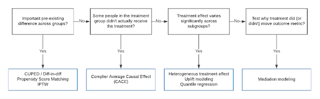
One important assumption this paper makes is that we've generated our training dataset from a randomized experiment! In other words, The potential outcomes $Y(1)$ and $Y(0)$ are independent from the treatment $W$. In this blog so far, we've focused mostly on causal inference in observational settings—when fundamental differences exist between the treatment and control group. In this paper, we assume the treatment and control groups are fundamentally the same but we have highly heterogeneous treatment effects—our treatment will have drastically different effects on different subsets of the population, and we need to make decisions in that context.
Evaluation ideas
Let's assume we've trained a model that solves this problem. How should we evaluate its quality?
Here is one way proposed by the researchers. We can draw inspiration from the the receiver operating characteristic curve, which plots the true positive rate against the false positive rate at various thresholds. For a highly-predictive model, the area underneath it will be close to 1. A model that guesses randomly has a ROC curve given by the dashed line from $(0, 0)$ to $(1, 1)$. (Note that this image comes from Wikipedia, not today's paper.)
 Similarly, in the context of maximizing retention while controlling cost, we can plot the incremental value gained by our model against its incremental cost. A high-quality model will capture much of the value when the cost is low; for a model that randomly picks users to include in the treat, incremental value will scale linearly with incremental cost. Like the AU-ROC curve, we can use the AUCC—the area under the cost curve—to evaluate our model's quality.
 Let's talk about models
Remember our end goal: we want to select the "best" set of users for our marketing promotion, subject to the constraint that we'd like to keep to a set budget. We can imagine this as a two-step process:


Shuyang Du, James Lee, Farzin Ghaffarizadeh
Here's the situation, handed to us in this paper from researchers at Uber: we'd like to offer a marketing promotion to our users in order to get them to retain better—to use our product more consistently over time. One way we can model this problem is with a binary random variable $Y^r$ (the $r$ stands for "retention"), where $Y_i^r = 1$ if and only if user $i$ used our product in a given time period. We could assume our marketing promotion has some fixed cost per user, then target the users with the highest treatment effect $\tau^r(x_i) = \mathbb{E}[Y_i^r(1) - Y_i^r(0) \mid X = x_i]$, where user $i$ has covariates $x_i$.
This might be a valid framing for some marketing promotions. For others, it is incomplete. Let's say for example you run, I don't know, a ride-sharing company, maybe we can call you Uber. One promotion you might run is to offer everyone free rides for a month. This will probably be great for user retention but not so great for the company bottom line!
A more complete framing of the problem might consider that our marketing intervention may also have an effect on the cost of a user to the business. Then if our marketing budget for this promotion is some number $B$, our objective is to maximize our promotions's effect on retention, subject to the constraint that we don't want to increase our costs more than $B$. We can use a second outcome variable $Y_i^c$ to indicate the cost of a user, and a second CATE function $\tau^c(x_i) = \mathbb{E}[Y_i^c(1) - Y_i^c(0) \mid X = x_i]$. Then, given a binary variable $z_i$ that indicates whether or not we'll pick a user to be in our treated group, we can fully frame the optimization problem we'd like to solve as follows:
$$\max \sum_{i=1}^n \tau^r(x_i)z_i \enspace s.t. \; \sum_{i=1}^n \tau^c(x_i)z_i \le B$$
One important assumption this paper makes is that we've generated our training dataset from a randomized experiment! In other words, The potential outcomes $Y(1)$ and $Y(0)$ are independent from the treatment $W$. In this blog so far, we've focused mostly on causal inference in observational settings—when fundamental differences exist between the treatment and control group. In this paper, we assume the treatment and control groups are fundamentally the same but we have highly heterogeneous treatment effects—our treatment will have drastically different effects on different subsets of the population, and we need to make decisions in that context.
Evaluation ideas
Let's assume we've trained a model that solves this problem. How should we evaluate its quality?
Here is one way proposed by the researchers. We can draw inspiration from the the receiver operating characteristic curve, which plots the true positive rate against the false positive rate at various thresholds. For a highly-predictive model, the area underneath it will be close to 1. A model that guesses randomly has a ROC curve given by the dashed line from $(0, 0)$ to $(1, 1)$. (Note that this image comes from Wikipedia, not today's paper.)


Remember our end goal: we want to select the "best" set of users for our marketing promotion, subject to the constraint that we'd like to keep to a set budget. We can imagine this as a two-step process:
- Produce a score $S_i$ for each user that represents how "good" of a target they are, i.e. how high the effect of the promotion on this user's retention is likely to be relative to the effect of the promotion on this user's cost.
- Target the set of users with the highest scores.
How should we produce $S_i$? Here's one idea: intuitively we'd like our scores to give a sense of "value per cost". To capture this, we can train two estimators $\hat{\tau}^r$ and $\hat{\tau}^c$ respectively, then let $S_i = \frac{\hat{\tau}^r(x_i)}{\hat{\tau}^c(x_i)}$.
The problem with this strategy is instability. Both estimators might be noisy, and the treatment effects on cost in the denominator might be quite small, which could cause problems in producing high-quality scores. To deal with this, the researchers construct a Lagrangian for the optimization problem:

Then (after some math), this optimization problem can be solved by picking users scored by $S_i = \hat{\tau}^r(x_i) - \lambda \hat{\tau}^c(x_i)$. We can then train a single estimator $\hat{\tau}^S$ on a new label $Y^S = Y^r - \lambda Y^c$, which solves our instability problem and allows us to only train and maintain one model instead of two. While it would be possible to iteratively learn a good value for $\lambda$, the researchers instead treat it as a hyper-parameter.
Ordinal prediction: a one-step process
Instead of picking users using the two step process above ("score with a model, then pick the best scores"), we could bake the concept picking of users into the model itself. This is the idea behind this paper's flagship algorithm, which the researchers term "Direct Ranking Model" (DRM).
Here's how it works. If we knew the probability $p_i$ that we would select sample i into our "best users" set, then we could compute the expected treatment effect on our selected users (notice that this math is only valid when the counterfactual outcomes are actually independent from the treatment—in the context of random experiments, in other words):
$$\mathbb{E}[Y^r(W = 1) - Y^r(W = 0) \mid X] $$
$$= \mathbb{E}[Y^r(W = 1) \mid X] - \mathbb{E}[Y^r(W = 0) \mid X]$$
$$ = \sum_{i=1}^n \mathbf{1}\{W_i = 1\} p_i Y_i^r - \sum_{i=1}^n \mathbf{1}\{W_i = 0\} p_i Y_i^r$$
So all we need to do is learn this probability $p_i$! We know how to do this: assume we have some differentiable scoring function that produces scores $S_i$. We can use the softmax function to turn this score into a probability (note that we actually have two softmax computations—one for treatment and one for control—which ensures that both expectation terms in the equation above are actually valid expectations):

Finally, since the scoring function is differentiable, we can learn it using off-the-shelf optimizers.
Evaluation and conclusion
The researchers evaluated their new algorithm on an offline dataset of about a million rides, and in an online setting. In both settings, the researcher's DRM algorithm performs better than their baseline models when it comes to efficiently increasing retention. Cool!

Further reading

Comments
Post a Comment